Simulations of investment strategies
Based on the ideas in a
blog
posting by Steven Landsburg (and the subsequent comments),
I did some simulations of various investment strategies. In all
cases, the basic assumptions are that we are investing for a fixed
number (N) of periods, and that during each period the investment grows
by a factor r which is normally distributed. For my simulations,
the number of periods is N = 15 and r has mean 1.05 and standard deviation 0.20,
so I'm thinking of each period as being a year and I've deliberately chosen r
to be volatile to emphasize the differences between the strategies.
The first two strategies are the two described in the blog entry,
which I've given descriptive names to here:
- step: ensure that at the start of the kth period,
the value of the investment is k dollars.
- steady: ensure that at the start of each period,
the value of the investment is (N+1)/2 dollars.
These two strategies have on average the same number of dollars
invested per period, so they have the same expected growth. But in the second,
the investments are spread more evenly over the periods, so the risk
is reduced.
Those two strategies are a bit unrealistic in that you can't predict
how much cash you need to have on hand in order to keep the investment
at the desired level. For example, if N = 3 (as Landsburg took), the
steady investor wants 2 dollars invested during each period. If it
happens that most of the investment is lost during each period, one
would need to invest 2 dollars each period for a total of 6 dollars.
If you have 6 dollars available for investing, then most of the time
it is better to have a larger investment, so you weren't doing the
right thing. (Of course, borrowing can help make this more realistic,
but I haven't included borrowing costs into this model.)
Two strategies that are more realistic are the following:
- dca: dollar cost averaging: each period, add one dollar
to the investment.
- lump: invest (N+1)/2 dollars at the start,
and make no changes after that.
The first is easily doable by someone who has a regular pay check and
can afford to invest a certain portion. The second is easily doable
by someone with some cash that is available for investing.
So, how do these four compare? With 15 periods and the rate for each
period independently drawn from a normal distribution with mean 1.05
and standard deviation 0.20, I ran one million trials. For each
trial, I took the value of the investment and subtracted the amount
invested (which in the case of step or steady depends on what happened
during the simulation). The results are:
  step:   6.00 +-  7.05  (118%)
  steady: 6.00 +-  6.20  (103%)
  dca:    7.66 +- 11.79  (154%)
  lump:   8.64 +- 13.98  (162%)
which displays the expected profit and the standard deviation of the
profit (also expressed as a percentage of the profit).
The 6.00 for the steady investor is easy to understand. He or she has
8 dollars invested during each period, and so on average earns 40
cents per period (5 percent of 8 dollars). Over 15 periods, that
totals to 6 dollars. As mentioned above, the step investor earns
on average the same amount, but with greater volatility.
But note that the strategies that are easier to accomplish (dca
and lump) in addition have a higher expected return!
This is because on average they have more invested.
Here is a plot of the distributions of profits for the four strategies
(with some long tails cut off). The vertical axis is an arbitrary
scale related to the density of the samples in the histogram bins.
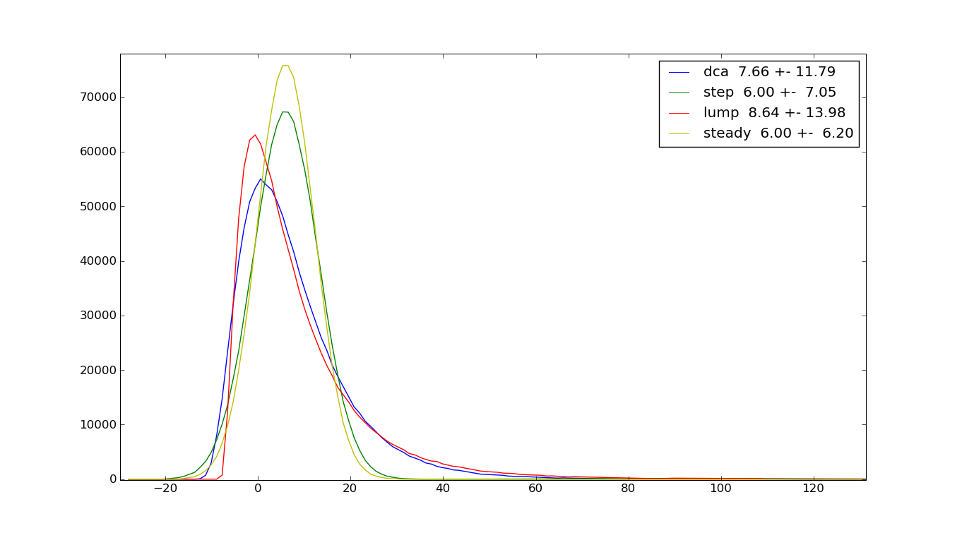
Note that dca and lump are more similar to each other than dca is to
step or lump is to steady. So it's not appropriate to use step and steady
as a way to argue whether dollar cost averaging is a reasonable
strategy. Indeed, step is clearly inferior to steady (if you have the
money upfront), whereas the decision between dca and lump depends on
your risk tolerance and other factors. In fact, the standard deviation of dca as a
percentage of the expected growth is less than that of lump,
meaning that by simply increasing the amounts invested, you can get
the same expected return as lump with less risk. Combined with the
fact that most individuals do not have their lifetime savings
available to invest early, dca comes out as a good strategy.
Similarly, one can argue that by increasing the amounts invested with
step or steady, one can get the same return as dca or lump with even
less risk. That is true, but it really only further reinforces the
point that dollar cost averaging is reasonable, since, for example, step
not only applies dollar cost averaging to the new investment made in
each period, but applies it to the investments made in previous
periods, either withdrawing profits or purchasing more to make up for
losses. It is that rebalancing that reduces the risk.
Conclusions
Here are the conclusions I draw:
- Dollar cost averaging (dca) reduces risk at the cost of reduced growth;
however, the reduction in risk is greater than the reduction in growth.
- The steady and step approaches reduce risk to an even greater
extent; however, they require reserves of capital that are
unrealistic. If you have the capital to invest, you are better off
investing it than holding it.
For most people, lump and steady are not realistic because they don't
have a large amount of cash to draw upon, and the above shows that
periodic investments of a fixed amount are a good thing to do.
If the investor does have a large amount of money to invest, and
wants to decide between investing all of it now, or doing it
over a fixed number of periods, then you should multiply the lump
results by 2N/(N+1) = 15/8 to get your comparison (because the lump
sum amount is now the sum of the periodic amounts):
  dca:    7.66 +- 11.79  (154%)
  lump:  16.20 +- 26.21  (162%)
Now you have a tough choice between large growth with large risk or small
growth with small risk...
Caveats
To be more realistic, a proper comparison would at least include an
alternative (less risky?) investment, a borrowing cost, and maybe a
set amount of cash on hand. Then one could try to optimize the
investing strategy using these constraints.
Comments and feedback welcome: Dan
Christensen <jdc@uwo.ca>
The code I used for these calculations is here: dca.py.